How Does Batch Normalization Help Optimization? 정리글

• Main Contribution
• Batch normalization and internal covariate shift
  • Does BatchNorm’s performance stem from controlling internal covariate shift?
  • Is BatchNorm reducing internal covariate shift?
• Why dose BatchNorm Work?
  • The smoothing effect of BatchNorm
  • Exploration of the optimization landscap
  • Is BatchNorm the best (only?) way to smoothen the landscape?
• Theoretical Analysis
  • Setup
  • Theoretical Results
    • Theorem 4.1 (The effect of BatchNorm on the Lipschitzness of the loss).
    • Theorem 4.2 (The effect of BN to smoothness).
    • Theorem 4.4 (Minimax bound on weight-space Lipschitzness).
    • Lemma 4.5 (BatchNorm leads to a favourable initialization).

Main Contribution

Batch normalization에 대하여에서 BN이 결국 internal covariate shift현상을 해결하여, 모델의 수렴속도를 높인다고 주장하였다. 하지만, 해당 논문에서는 internal covariate shift현상을 감소하여 그러는 것이 아니며, BN이 실제로 감소시키지 않는다고 주장한다.

이 논문에서는 BN이 optimization problem을 smoother하게 만들어서 성공적이라고 주장한다. 이로 인해서 gradient는 predictive해지고 더 큰 learning rate를 사용할 수 있다.

optimization problem이 smoother 해진다는 것은…

https://ifm.mathematik.uni-wuerzburg.de/~schmidt/publications.php

Batch normalization and internal covariate shift

train, test 그래프에서는 batch normalization의 역할을 잘 보여주고 있다. 높은 learning rate를 사용할 수 있는 것을 보여주고 있는데, 오른쪽의 그래프를 보면 BN을 적용한 모델의 activation과 그렇지 않은 모델의 activation의 분포가 그리 큰 차이를 가지고 있지 않는 것을 확인 할 수 있다. 이런 결과를 가지고 다음과 같은 질문을 할 수 있다.

• Batch Normalization의 효과가 internal covariate shift와 연관이 있는 것인가?
• Batch Normalization이 internal covariate shift를 감소시키는 역할을 하는가?

Does BatchNorm’s performance stem from controlling internal covariate shift?

layer input의 distribution의 mean, variance를 조정하는 것이 training performance를 향상시킬 수 있는것 인가? 이를 어떻게 입증할 것인가?

다음과 같은 실험환경을 구성하였다.

• BN을 적용한 후, $random$ noise를 추가하였다. 이 noise는 non-zero mean을 가지며 non-unit variance distribution이다. 또한 training step마다 noise distribution은 바뀐다.
• noise가 추가되면 결국 covariate shift현상이 생기는 것이다.

위의 그림을 보면, Standard + BatchNorm과 Standard + ‘noisy’BatchNorm과의 성능 차이가 거의 없음을 알 수 있다. 즉, internal covariate shift를 해결하는 것과 batch normalization의 효과를 무관하다고 볼 수 있다. 또한 오른쪽 이미지를 보면, Standard + ‘noisy’BatchNormdl Standard보다 덜 안정적인 distribution을 가지고 있는 것을 확인할 수 있다. 하지만, 실험결과는 Standard + ‘noisy’BatchNorm이 우수한 걸로 보아 stable distribution이 training performance에 주는 영향은 미비한 것으로 보인다. 또한 Standard에 noise를 섞을 때, 전혀 학습이 안되는 것을 확인할 수 있었다.

결국 internal covariate shift를 감소시키는 것과 batch normalization효과는 관련이 있다고 보기 힘들다.

Is BatchNorm reducing internal covariate shift?

위에서 internal covariate shift와 training performance와 직접적인 관계가 없다는 것을 증명했다. 하지만, 보다 넓은 관점에서의 training performance와 연관된 internal covariate shift(ICS)이 있을까라는 궁금증이 들 수 있으며, 만약 그렇다면 BatchNorm은 ICS를 감소시킬까?

각 layer는 empirical risk minimization을 수행하고 있다. 만약 layer가 학습도중에 update된다면, 이전 layer가 변하기 때문에 input도 변한다.

empirical risk minimization

• risk란 loss function의 expectation을 의미한다.

$$R(h) = \int L(f(x), y) dP(x, y)$$

Is BatchNorm reducing internal covariate shift? 이 질문에 답하기 위해서는 더 넓은 개념의 internal covariate shift를 다뤄야 한다. 이는 optimization problem과 연관이 깊다. 일반적으로 training은 first-order method를 사용하기 때문의 loss의 gradient는 친숙한 편이다. layer내의 parameters가 이전 layer의 update영향으로 얼마큼 조정해야하는지 측정하기 위해서는 이전 layer가 update되기 전과 후의 gradient간의 차이를 구해야한다.

Notation

• loss: $\mathcal{L}$

• $k$ layers의 parameters(time = t): $W_1^{(t)}, W_2^{(t)}, \cdots W_k{(t)} $

• batch of input-label pairs(time = t):$(x^{(t)}, y^{(t)})$

• internal covariate shift =$\rVert G_{t, i} - \acute{G_{t, i}}\rVert_2 $ $G_{t, i} = \nabla_{W_i^{(t)}}\mathcal{L(W_1^{(t)}, W_2^{(t)}, \cdots W_k^{(t)} ;x^{(t), y^{(t)}} )}$

  $$\acute{G_{t, i}} = \nabla_{W_i^{(t+1)}}\mathcal{L(W_1^{(t+1)}, \cdots W_ {i-1}^{(t+1)},W_ {i}^{(t)}, W_ {i+1}^{(t)} \cdots W_k^{(t)} ;x^{(t), y^{(t)}} )}$$

위의 internal covariate shift 산출방법으로 bath norm을 적용한 경우와 그렇지 않은 경우를 비교하였다. 이전의 주장은 BN이 ICS를 감소시킨다고 주장하였으나, 실험결과 BN이 ICS를 증가시키기도 하였다. 위의 그림을 보면 확인 할 수 있다. 이런 현상은 DLN에서 더 도드라 진다. DLN을 보면 오히려 Standard한 것이 ICS가 적게 나타나는데 비해서 BN을 적용할 때는 $G, \acute{G}$는 서로 상관관계가 없어보인다. (하지만 training 결과는 loss, acc 측면에서 더 좋게 나온다.)

결국 batch normalization은 internal covariate shift를 감소시키지 않는다는 것을 증명하였다.

Why dose BatchNorm Work?

위에서 밝혔듯이 BatchNorm과 ICS는 관련이 없다. 하지만, BatchNorm은 exploding gradient 혹은 vanishing gradient 문제에 있어서 효과적이다. 하지만 이는 BatchNorm이 training performance를 향상 시키는 본질적인 이유라고 할 수 없다.

The smoothing effect of BatchNorm

it reparametrizes the underlying optimization problem to make its landscape significantly more smooth.

결론부터 말하면, BatchNorm은 optimization 문제를 smooth하게 바꾸어 training performance를 개선시키고 있다.

그 이유는 loss function의 Lipschitzness 를 개선시키기 때문이다.

gradient의 변화가 loss의 변화보다 적은 상태, 따라서 loss가 작은 learning rate로 변하게 되면 gradient도 작게 변하게 된다.

$f$ is L-Lipschitz if $\rvert f(x_1) - f(x_2) \rvert \le L\rVert x_1-x_2\rVert $ for all $x_1, x_2$

이 특성은 BatchNorm의 reparameterization을 만나게 되면 더 커지는데, loss는 effective한 $\beta$-smoothness 효과를 가지게 된다. 아래의 그래프에서 확인 할 수 있다.

$\beta$-smoothness란?

Recall that f is β-smooth if its gradient is β-Lipschitz

$$\rvert f(x) -f(y) - \nabla f(y)^T(x- y)\rvert \le \frac{\beta}{2}\rVert x-y\rVert^2$$

https://arxiv.org/pdf/1405.4980.pdf

이 smooth 효과는 training algorithm에 매우 효과적이다. non-BatchNorm의 loss function은 non-convex할 뿐만 아니라 kinks, flat regions , sharp minima의 문제를 가지고 있다. 이 문제는 gradient 방법론이 수렴하기 불안정하도록 만든다. 하지만 BatchNorm을 적용하게 되면, gradient가 reliable하고 predictive한 방향으로 나오게 된다. 무엇보다도 개선된 Lipschitzness는 learning step을 크게 잡을 수 있게 해준다. 아래의 그래프를 보면 그 효과를 확인할 수 있다.

Exploration of the optimization landscap

위의 그래프의 Figure 4(a)를 보면 step마다의 loss변화를 알 수 있다. 이를 통해서 non-BatchNorm의 방식은 loss의 변화량이 BatchNorm보다 크다는 것을 알 수 있다. 이런 현상은 초기 학습과정에서 특히 심하다.

또한 gradient의 predictiveness도 살펴볼수 있다. Figure 4(b)를 보면, 이를 확인할 수 있는데, predictiveness는 주어진 시점에서의 loss gradient와 다른 시점에서의 loss gradient간의 $l_2$ distance로 정의하였다.

Figure 4(c)에서는 BatchNorm의 loss gradient stability/Lipschitzness의 향상을 확인할 수 있다. 이는 gradient direction 뿐만 아니라, random direction에 대해서도 결과가 유사하게 나왔다.

Is BatchNorm the best (only?) way to smoothen the landscape?

실험결과 $l_1$ normalization의 결과가 BatchNorm보다 좋게 나왔다. 기억할 것은 $l_p$ normalization은 distribution shift를 일으킨다는 것이다. 하지만, 여전히 성능을 향상 시킨다. (결국, ICS와 성능향상은 무관하다는 것이다.)

아래의 실험결과를 보면, 꼭 BatchNorm을 고집할 이유는 없어 보인다.

Theoretical Analysis

Setup

fully-connected layer W에 single BatchNorm을 추가한 효과를 분석하고자 한다. Figure 5(b)와 같은 상황을 가정한다. 주목할 점은 input에 BatchNorm을 적용한 것이 아니라, layer W의 output에 BatchNorm을 적용한다. 이는 해당 논문의 분석이 단지 input에 대한 normalization 효과에 대한 것이 아니라 reparameterization에 대한 것임을 알려준다.

Notation

• layer weights: $W_{ij}$
• Figure 5(a) network와 Figure 5(b) network는 모두 동일한 loss function을 가지고 있다. (loss function내부에는 non-linear layer들이 추가적으로 있을 수 있다.)
• BatchNorm loss: $\hat{\mathcal{L}}$
• 위의 두 network모두 input $x$과 activation $y = Wx$를 가진다. BatchNorm의 경우에는 $\hat{y}$를 추가적으로 가지게 되는데 이는 normalized된 activation이다.(mean=0, var=1)
• $\gamma, \beta$는 모두 constant라고 가정한다.
• $\sigma_j$는 batch의 output $y_i \in R^m$의 stadard deviation이다.

Theoretical Results

activation $y_i$에 대한 optimization landscape를 생각해보자. 앞서 BatchNorm이 결국 landscape가 더 잘 작동하도록 만든다는 것을 실험을 통해 증명하였다. (Lipschitz-continuity, and predictability of the gradients ) 이 논문에서는 activation-space상에서 landscape가 weight -space landscape에서의 worst-case bounds가 된다는 것을 증명할 것이다.

gradient magnitude $\rVert\nabla_{y_i}\mathcal{L}\rVert$에 대해서 먼저 생각해보자. 이는 Lipschitzness를 나타내주는 지표이다. loss의Lipschitzness는 optimization문제에서 큰 역할을 한다고 알려져 있다. (이 지표는 결국 loss가 training step에 따라서 얼마나 변할지 알려주기 때문)

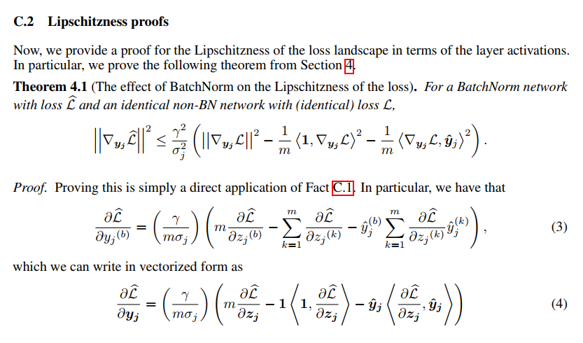
Theorem 4.1 (The effect of BatchNorm on the Lipschitzness of the loss).

For a BatchNorm network with loss $\hat{\mathcal{L}}$ and an identical non-BN network with (identical) loss $\mathcal{L}$,

$$\rVert\nabla_{y_i}\mathcal{L}\rVert^2 \le \frac{\gamma^2}{\sigma_j^2}\left( \rVert\nabla_{y_i}\mathcal{L}\rVert^2 - \frac{1}{m} \left\langle 1, \nabla_{y_i}\mathcal{L}\right\rangle ^ 2 - \frac{1}{m}\left\langle \nabla_{y_i}\mathcal{L}, \hat{y}_j\right\rangle ^ 2 \right)$$

해당 논문에서는 어떤 가정도 없이 BatchNorm이 더 개선된 Lipschitzness를 가진다고 증명하였다. 게다가 Lipschitz constant는 normalized activation $\hat{y}$가 gradient $\nabla_{y_i}\mathcal{L}$ 혹은 0에서의 gradient deviates값의 mean값과 상관관계가 있을 때 감소되는 것을 확인할 수 있었다. 이 효과는 BN의 scaling이 기존 layer의 scaling과 일치할 때도 나타났다. 아래는 appendix에서 가져온 것이다.

Fact C.1 Gradient throgh BatchNorm

notation

• gradient through BN: $\frac{\partial f}{\partial A^{(b)}}$
• another function:$f := f(C) $ where $C = \gamma \cdot B + \beta$ and $B = BN_{0, 1}(A) := \frac{A-u}{\sigma}$
• scalar elements of a batch size of size m and variance $\sigma^2$: $A^{(b)}$

$$\frac{\partial f}{\partial A^{(b)}} =\frac{\gamma}{m\sigma}\left( m\frac{\partial f}{\partial C^{(b)}} - \sum_{k=1}^{m}\frac{\partial f}{\partial C_{(k)}} - B^{(b)}\sum_{k=1}^{m}\frac{\partial f}{\partial C_{(k)}}B^{(k)}\right)$$

Fact C.2 Gradient of normalized outputs

convenient gradient of BN $\frac{\partial \hat{y}^{(b)}}{\partial y^{(k)}} = \frac{1}{\sigma}\left(1[b=k] =\frac{1}{m} - \frac{1}{m}\hat{y}^{(b)}\hat{y}^{(k)}\ \right)$ 그러므로, $\frac}{\partial y^{(k)}} = \frac{\gamma}{\sigma}\left(1[b=k] =\frac{1}{m} - \frac{1}{m}\hat{y}^{(b)}\hat{y}^{(k)}\ \right)$

$\left\langle 1, \nabla_{y_i}\mathcal{L}\right\rangle ^ 2$ 은 해당 차원에서 quadratically하게 증가한다. 그러므로 중요한 term이다. 게다가 $\left\langle \nabla_{y_i}\mathcal{L}, \hat{y}_j\right\rangle ^ 2$은 zero 값으로 부터 조금 떨어진 값이라고 기대되는데 이는 variable과 variable의 gradient term이 일반적으로 uncorrelated하기 때문이다. $\sigma_j$는 커지는 경향이 있는데$\gamma $-scaling을 해줌으로써 flatness가 되도록 해주는 효과를 기대할 수 있다.

proof

Fact C.1을 이용하여 다음과 같이 전개한다.

자세한 증명은 해당 논문의 appendix를 참고하길 바란다.

Theorem 4.2 (The effect of BN to smoothness).

**Let $\hat{g}i = \nabla{y_i}\mathcal{L}$ and $H_{j j} = \frac{\partial\mathcal{L}}{\partial{y_i}\partial{y_i}}$ be the gradient and Hessian of the loss with respect to the layer outputs respectively. Then ** $\left( \nabla_{y_i}\hat{\mathcal{L}} \right)^T\frac{\partial\hat{\mathcal{L}}}{\partial{y_i}\partial{y_i}} \left( \nabla_{y_i}\hat{\mathcal{L}}\right) \le \frac{\gamma^2}{\sigma_j^2} \left(\frac{\partial\hat{\mathcal{L}}}{\partial{y_i}} \right) H_{jj} \left(\frac{\partial\mathcal{L}}{\partial{y_i}} \right) - \frac{\gamma}{m\sigma^2} \left\langle \hat{g_j}, \hat{y_j} \right\rangle \rVert\frac{\partial\mathcal{L}}{\partial{y_i}} \rVert^2$

만약,$\hat{g_j}, \nabla_{y_i}\hat{\mathcal{L}}$의 relative norm을 보존하는 $H_{jj}$를 가지고 있다면?

$$\left( \nabla_{y_i}\hat{\mathcal{L}} \right)^T\frac{\partial\hat{\mathcal{L}}}{\partial{y_i}\partial{y_i}} \left( \nabla_{y_i}\hat{\mathcal{L}}\right) \le \frac{\gamma^2}{\sigma_j^2} \left( \hat{g_i}^TH_{jj}\hat{g}_i - \frac{1}{m\gamma} \left\langle\hat{g_j}, \hat{y_j} \right\rangle\right)\rVert\frac{\partial\mathcal{L}}{\partial{y_i}} \rVert^2$$

이제 landscape의 second-order 특성을 살펴보자. BatchNorm이 더해지면, loss Hessian(gradient direction에 대한 activation에 대한 hessian)은 input variance에 의해서 rescaled되고 increasing smoothness에 의해서 감소하게 된다. 이는 Taylor expansion에 의해서 도출할 수 있으며, 이 term을 감소시키는 것은 gradient가 더 predictive한 성격을 가지게 한다.

$\left\langle \hat{y_j},\hat{g_j}\right\rangle$이 non-negative 한 성격을 가지고 Hessian을 가진다면, 위의 theorem은 더 예측가능한 gradient값을 가진다.(predictive gradient) Hessian은 loss가 locally convex하게 되면, positive semi-definite한 성격을 가지게 된다.

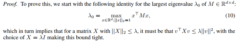
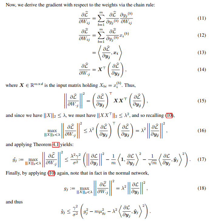
Theorem 4.4 (Minimax bound on weight-space Lipschitzness).

For a BatchNorm network with loss $\hat{\mathcal{L}}$ and an identical non-BN network (with identical loss $\mathcal{L}$), if

여기서는 BatchNorm이 layer weights에 대한 worst-case bound역할을 하는 것을 보일 것이다. $g_j = \max_{\rVert X \rVert \le \lambda}\rVert \nabla_W\mathcal{L}\rVert^2$

$$\hat{g_j} = \max_{\rVert X \rVert \le \lambda}\rVert \nabla_W\hat{\mathcal{L}}\rVert^2 \Rightarrow \hat{g}_j \le \frac{\gamma}{\sigma_j^2}\left( g_j^2 - mu^2_{g_j} -\lambda^2\left\langle \nabla_{y_j}\mathcal{L}, \hat{y}_j\right\rangle^2 \right)$$

아래는 이에 대한 증명이다.

Lemma 4.5 (BatchNorm leads to a favourable initialization).

*Let $W^$ and $\hat{W}^*$ be the set of local optima for the weights in the normal and BN networks, respectively. For any initialization $W_0$ **

initialization에서도 성능 향상이 있었다.

Reference

• https://arxiv.org/abs/1805.11604