Determinant and Trace 정리글
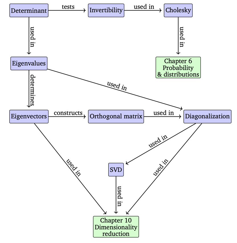
Matrix Decomposition
matrix는 linear mapping을 나타낼 수도 있지만, 데이터 자체를 표현하는데 사용되기도 한다. 이번 장에서는 matrix가 요약되고, decompostion되며 그리고 이를 통해서 matrix approximation에 대해서 다룰 것이다.
matrix를 몇 가지 숫자로 묘사할 수 있는데, determinant와 eigenvalue를 보면 알 수 있다. 이번 장에서 아래와 같은 마인드맵을 참고하면서 공부하면 큰 그림을 그리는데 도움이 될 것이다.
Determinant
determinant는 system of linear equation과 연관이 깊다. 그리고 아래와 같이 기호로 나타낸다. determinant는 $n \times n$ matrix꼴에서만 정의된다.
Invertibility
Theorem 4.1. For any square matrix $A \in R^{n \timers n}$ it holds that A is invertible if and only if $det(A) \neq 0$.
-
$T_{ij} = 0, \forall i > ji$: upper trianglar matrix
-
$T_{ij} = 0, \forall i < ji$: upper trianglar matrix
-
T는 trianglar matrix
Example 4.2 Determinant as Measures of Volume
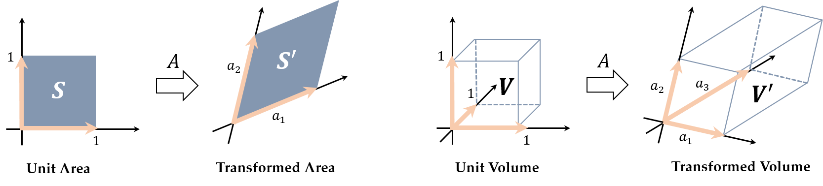
linear mapping에 대해서 생각해보자. linear mapping은 결국 basis change를 하는 것이다.
예를 들어서, 어떤 vector에 linear mapping을 하게되면 위의 그림 처럼 basis가 unit vector에서 변화가 생기게 된다. 이 때 determinant는 각 basis가 이루는 volume이며, 위의 그림처럼 volume의 변화가 생긴다.
- reference:
- https://emoy.net/Determinant
- https://www.youtube.com/watch?v=Ip3X9LOh2dk&ab_channel=3Blue1Brown
Compute Determinant
Theorem 4.2 (Laplace Expansion) consider a matrix $A \in R^(n \times n)$, for all $j = 1, \cdots, n$
-
Expansion along column j
-
Expansion along row j

The Properties of Determinant
- $det(AB) = det(A)det(B)$
- $det(A) = det(A^T)$
- A is invertible(regular) if $det(A) \neq 0$
- similar Matrices는 서로 같은 determinatn를 가진다.
- $\hat{A} = S^{-1}AS$
- matrix내의 한 row/col에 다른 row/col을 더하는 것은 det(A)에 영향을 주지 않는다.
- 이 특징을 활용하여, gaussian elimination을 진행하여, traianglar matrix형태로 만들 수 있다.
- $det(\lambda A) = \lambda^n det(A)$
- column이나 row의 순서를 바꾸면 det(A)의 부호가 바뀔 수 있다.
Theorem 4.3 A square matrix $A \in R^{n \times n}$
Trace
The trace of square matrix $A \in R^{n \time n}$ is defined as
-
tr(A + B) =$tr(A) + tr(B) \forall A, B \in R^{n \time n}$
-
$tr(\lambda A) = \lambda tr(A), \text{ for } \lambda \in R, A \in R ^{n \time n}$
-
$tr(I_n) = n$
-
$tr(AB) = tr(BA) \text{ for } A \in {R^{n \times k}, B \in R^{k \times n}}$
similar matrix
Characteristic Polynomial
For $\lambda \in R, A \in R^{n \times n}$