Conjugacy and the Exponential Family 개요
머신러닝 관점에서는 확률분포에 대해서 다음과 같은 특징들이 중요하다.
- Closure Property: 한 집합의 원소끼리 특정 연산한 결과가 같은 집합에 있는 것이 보장
- Data를 더 수집해도 필요한 파라미터는 변하지 않는다.
- 좋은 파라미터를 원함.
Exponential Family라고 불리는 확률분포는 계산상 이점과 인퍼런스시 이점을 가지고 있다.
Exponential Family를 살펴보기전에 베르누이분포, 이항분포, 베타분포에 대해서 살펴볼 것이다.
베르누이분포
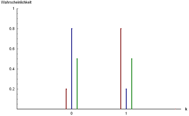
이항분포

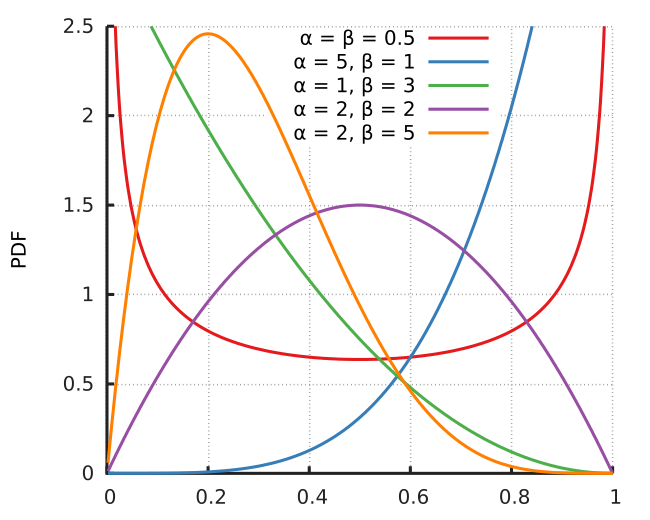
베타분포
Conjugacy
Bayes Theorem에 의하면 Posterior는 Prior와 Likelihood의 곱으로 이루어진다.
Prior를 고르는 것은 아래 두 가지 이유 때문에 힘들다.
- Prior는 문제에 대해 가지고 있는 지식을 가지고 있어야한다.
- Posterior를 계산하기 힘들다.
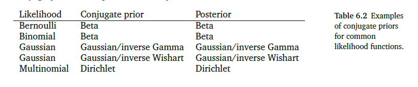
하지만 계산상 이점이 있는 분포가 존재하며 이를 Conjugacy Prior라고 한다.
Definition: Conjugacy Prior
Posterior가 Prior와 같은 분포이면 Prior는 Likelihood에 대해서 Conjugate이다.
Conjugate는 Posterior를 파라미터를 업데이트 시킴으로써 구할 수 있으며 이는 매우 편리하다.
Beta-Binomial Conjugacy
다음과 같은 Binomial Distribution $x \sim Bin(N, u)$을 고려해보자.
p(x∣N,u)=(Nx)ux(1−u)N−x,x=1,⋯,N
그리고 다음과 같은 Beta Prior가 있다고 해보자.
p(u∣α,β)=Γ(α)Γ(β)Γ(α+β)uα−1(1−u)β−1
Posterior 분포는 다음과 같이 구할 수 있다.
p(u∣x=h,N,α,β)∝p(x∣N,u)p(u∣α,β)∝uh(1−u)N−huα−1(1−u)β−1∝uh+α−1(1−u)N−h+β−1
Beta-Bernoulli Conjugacy
- $x \in {0, 1}$
- $\theta \in [0, 1]$
- $p(x=1 \mid \theta) = \theta$
- $p(x \mid \theta) = \theta^x (1- \theta)^{1 - x}$
- Prior: $p(\theta \mid \alpha, \beta) \propto \theta^{\alpha - 1} (1 - \theta)^{\beta - 1}$
p(θ∣α,β)=p(x∣θ)p(θ∣α,β)∝θx(1−θ)1−xθα−1(1−θ)β−1=θx+α−1(1−θ)β+(1−x)+1∝p(θ∣α+x,β+(1−x))
Conjugacy Table
Sufficient Statistics
Random Variable의 통계값이 Constant라는 것을 생각해보자.
Sufficient Statistics는 데이터로 부터 얻을 수 있는 정보를 모두 포함한 Statistics이다.
즉 Sufficient Statistics는 분포를 재현할 수 있다.
다음 예를 살펴보자.
- $X \sim p(x \mid \theta)$: Random Variable X는 $\theta$에 영향을 받음
Vector $\phi (x)$가 $\theta$에 대한 모든 정보를 가지고 있다면 Sufficient Statistics라고 한다.
즉 오직 $\phi (x)$에 의해서 $\theta$에 의존적인 부분과 독립적인 부분을 Factorize할 수 있다.
Theorem: Fisher-Neyman
$\phi (\theta)$는 $p(x \mid \theta)$를 아래와 같이 표현할 수 있을때 Sufficient Statistics라고 한다. (if and only if)
p(x∣θ)=h(x)gθ(ϕ(x))
- $h$: $\theta$와 독립
- $g_{theta}$: Sufficient Statistics $\theta(x)$에 의한 모든 의존성을 가지고 있음
만약 $p(x \mid \theta)$가 $\theta$와 독립이라면, $\phi (\theta)$는 어떤 $\phi$에 대해서도 Trivial Sufficient Statistics가 된다.
재밌는 경우는 $p(x \mid \theta)$가 $x$에는 독립이고 $\phi(x)$에 대해서는 의존적인 경우이다. 이 경우에는 $\phi(x)$는 $\theta$에 대한 Sufficient Statistics이다.
머신러닝에서는 한정된 수의 샘플을 가지고 분포를 추정한다.
더 많은 데이터가 있으면 더 일반적인 분포를 추정할 수 있다.
하지만 더 많은 파라미터가 필요하다.
그렇다면 이런 질문도 가능하다.
어떤 분포가 한정된 차원의 Sufficient Statistics를 가질 수 있는가?
정답은 Exponential Family이다.
Exponential Family
확률분포를 고려할 때 3단계의 추상화 과정이 있다.
- 파라미터와 분포의 종류가 정해짐.
- 분포의 종류는 정해졌으나 파라미터는 정해지지 않음
- 분포의 Family를 고려 (Exponential Family)
Exponential Family는 확률분포의 Family이다.
이 때 Family는 파라미터 $\theta \in R^D$를 가진다.
- $\phi(x)$: Sufficient Statistics Vector
p(x∣θ)=h(x)exp(<θ,ϕ(x)>−A(θ))
p(x∣θ)∝exp(<θ,ϕ(x)>)
Example: Gaussian as Exponentail Family
- $\mathcal{N}(u, \sigma^2)$
- $\phi(x) = \begin{bmatrix} x \ x^2\end{bmatrix}$
p(x∣θ)∝exp(θ1x+θ2x2)
θ=[σ2u−2σ21]T
θ∝exp(σ2ux−2σ2x2)∝exp(−2σ21(x−u)2)
Example: Bernoulli as Exponential Family
p(x∣u)=ux(1−u)1−x,x∈{0,1}
p(x∣u)=exp[logux(1−u)1−x]=exp[xlogu+(1−x)log(1−u)]=exp[xlogu−xlog(1−u)+log(1−u)]=exp[xlog1−uu+log(1−u)]
h(x)=1θ=log1−uuϕ(x)=xA(θ)=−log(1−u)=log(1+exp(θ))
u=1+exp(−θ)1