eigenvalue 와 enginevector 정리글
- Eigenvalue 와 Eigenvector
- Definition 4.6
- Definition 4.7 (collinearity and codirection)
- Remark: non-uniqueness of eigenvector
- Theorem 4.8
- Definition 4.9
- Definition 4.10 (Eigenspace and Eigenspectrum)
- Useful Properties of eigenvalue and eigenvector
- Example 4.5
- Definition 4.11
- Geometric Intuition in Two Dimensions
- Theorem 4.12
- Definition 4.13
- Theorem 4.14
- Theorem 4.15 (spectral theorem)
- Theorem 4.16
- Theorem 4.17
Eigenvalue 와 Eigenvector
Definition 4.6
square matrix $A \in R^{n \times n}$가 주어졌을 때, 아래의 식을 만족하면 $\lambda \in R$는 engienvalue이고 $x \in R^n/{ 0}$는 eigenvector 이다. 그리고 아래의 식을 eigenvalue equation이라고 한다.
아래의 명제들은 모두 동치이다.
- $\lamdba \in R$ 은 eigenvalue이다.
- $Ax = \lambda x$ 혹은 $(A -\lambda I)x = 0$의 해가 non-trivialy하다. ($x \in R ^ n / {0}$)
- $rk(A -\lambda I) < n$: eigenvector x가 non-trivial한 해이므로
- $det(A -\lambda I) = 0$
Definition 4.7 (collinearity and codirection)
두 vector가 같은 방향인 것을 codirection, 반대인 것을 colinearity라고 정의한다.
Remark: non-uniqueness of eigenvector
- $c \in R/ {0}$
- $x \ in R^n$: eigenvector
Theorem 4.8
$\lambda$ 는 characteristic polynomial $p_A(\lambda)$ of A의 해일 때만, eigenvalue이다.
이는 $(A - \lambda I) x = 0$에서 $A - \lambda I$가 0 vector가 아닌 해를 가져야 하기 때문이다.
Definition 4.9
square matrix A가 eigenvalue $\lambda$를 가진다고 가정해보자.
$\lambda$의 algebraric multiplicity는 동일한 eigenvalue와 대응하는 eigenvector의 수이다.
Definition 4.10 (Eigenspace and Eigenspectrum)
- Eigenspace: 모든 eigenvector들로 span 되는 공간
- Eigenspectrum: 모든 eigenvalue의 집합
Useful Properties of eigenvalue and eigenvector
-
$A, A^T$는 동일한 eigenvalue를 가지지만, eigenvector는 꼭 그렇지 않다.
-
similar matrices는 모두 동일한 eigenvalue를 가진다. 따라서, linear mapping $\Phi$는 basis 선택과 독립적인 eigenvalue를 가진다고 해석할 수 있다.
- Symmetric, positive matrix는 항상 실수의 eigenvalue값을 가진다.
Example 4.5
Definition 4.11
$\lambda_i$를 square matrix A의 eigenvalue라고 가정하자. 이때 $\lambda_i$의 geometric multiplicity는 eigenvalue $\lambda_i$와 연관되는 linear independent eigenvector들의 수이다.
따라서, eigenvalue의 algebraric multiplicity는 geometric multiplicity보다 항상 크거나 같다.
Geometric Intuition in Two Dimensions
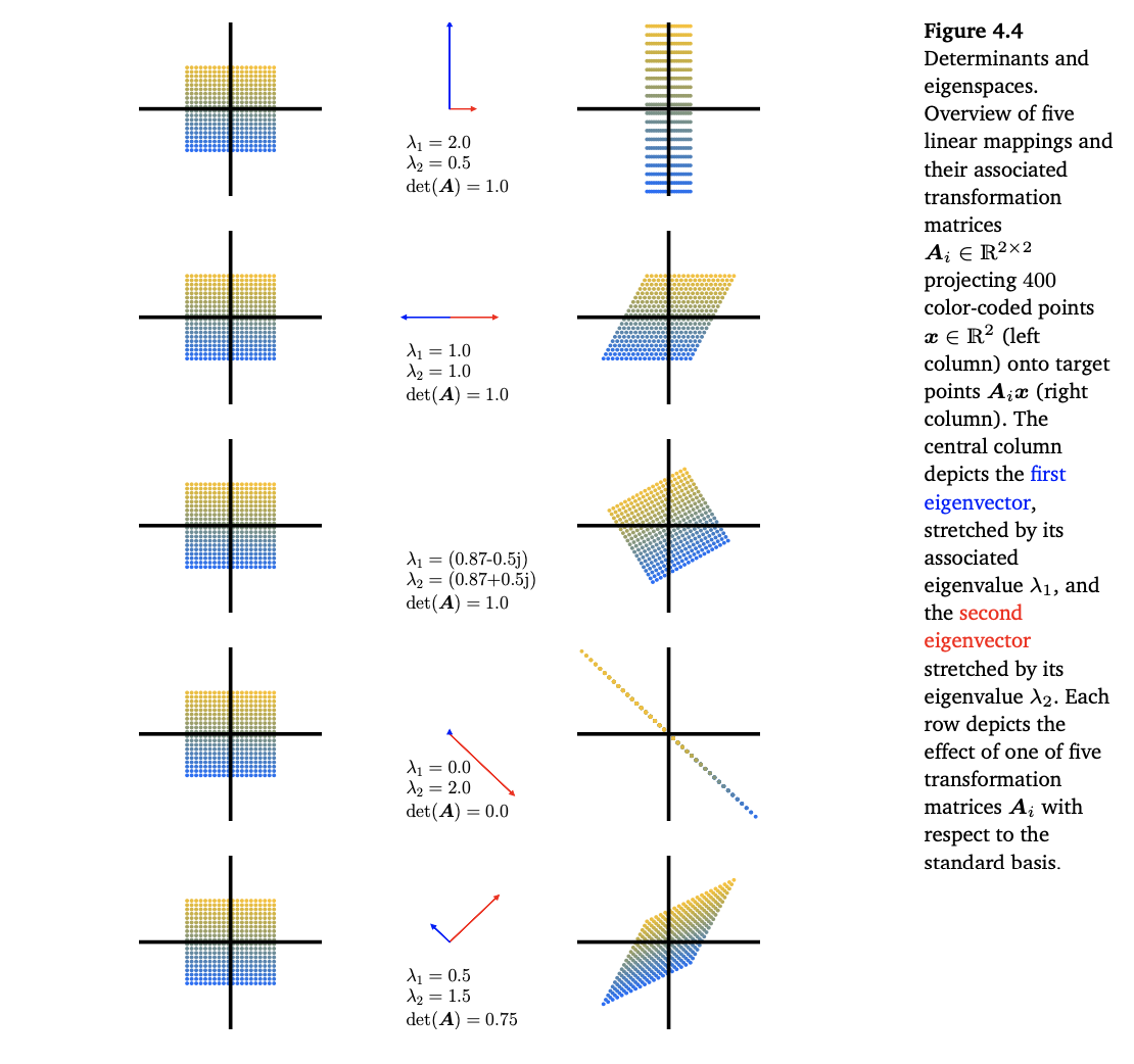
아래의 이미지는 각 linear mapping에 대해서 eigenvalue, eigenvector, determinant등의 정보를 시각화한 것이다.
주목할 점은 sqaure matrix A의 eigenvector v는 A linear mapping을 적용해도, norm만 달라질뿐, vector의 방향은 바뀌지 않는다. 또한 eigenvalue는 $det(A - \lambda I) = 0$의 해이다.
-
첫 번째 이미지는 아래와 같은 linear mapping을 시각화 한 것이다. 어떤 vector x에 linear mapping을 적용하면, $Ax$가 되며 이를 우측의 이미지와 같이 표현했다.
해당 linear mapping은 x축으로는 압축하는 형태로 y축은 확장하는 형태이다. 따라서 eigenvector는 위의 이미지 같이 나오며, 각각의 eigenvalue는 characteristic polynomial의 해로 구할 수 있다.
determinant는 1이다.
-
두 번째 이미지는 아래와 같은 linear mapping을 시각화한 것이다. shearing이라고 볼 수 있다.
이미지처럼 기울인 효과가 있으며, 직관적으로 $[0, 1]$ 성분이 조금이라도 있다면 방향이 바뀌므로 eigenvector는 x축 위에 있어야 한다는 것을 알 수 있다.
A의 eigenvalue는 $\lambda_1 = \lambda_2 = 1$이므로, 한 eigenvalue에 중복되는 eigenvecor가 대응된다.
determinant는 1로 위와 동일하다.
-
세 번째 이미지는 아래와 같은 linear mapping을 시각화 한 것이며, rotation이다.
어떤 vector도 A에 의해서 방향이 바뀌므로, eigenvector는 존재할 수 없으며 eigenvalue는 complex(허수)이다. 또한 volume을 그대로 유지하므로 determinant는 1이다.
-
네 번째 이미지는 2차원 공간을 1차원 공간으로 뭉개는 linear mapping이다.
공간을 뭉개기 때문에, determiant는 0이다.
eigenvector는 뭉개져서 mapping되는 1차원 선위에 위치해야 방향성이 유지 된다. 그리고 eigenvalue 중 하나가 0이 나오므로, 하나의 eigenvector는 뭉개진다.
-
다섯 번째 이미지는 shear-and-strecth mapping이다.
determiant는 0.75로 직관적으로 volumne이 0.75배되었다고 해석할 수 있다. 위의 이미지처럼 각 대각선 방향의 eigenvector는 linear mapping이 진행되어도 방향은 동일한 것을 직관적으로 알 수 있다.
Theorem 4.12
Distinct eigenvalue와 대응되는 eigenvector들은 서로 linear independent하다.
Proof
- $lambda_1, \cdots, \lambda_n$: distinct eigenvalues
- $v_1, \cdots, v_n$: 위의 eigenvalue와 대응되는 eigenvector들
아래 식의 해가 $c_1 = \cdots = c_n = 0$뿐이라면, $v_0, \cdots, v_n$은 서로 linear independent하다.
이를 이용하여, 증명을 진행해보자.
위의 식에 양변에 $\lambda_1$을 곱하면,
위의 식에 양변에 $A$를 적용하면,
위의 두개의 식을 빼면,
$\lambda_2 - lambda_1$는 0이 아니고, $v_2$도 0 vector가 아니므로 $c_2 = 0$ 이 된다. 이런 방식으로 다른 eigenvector에 적용하게 되면 모두 $c_i = 0$의 해만 가지게 된다. 따라서 distinct eigenvalue와 대응되는 eigenvector는 서로 linear independent하다.
Definition 4.13
Square matrix $A \in R^{n \times n}$는 linear independent한 eigenvector의 수가 n보다 적다면, defective하다고 한다.
Theorem 4.14
Matrix $A \in R ^{m \times n}$이 주어졌을 때, 항상 다음과 같은 positive semidefinite, symmetric한 matrix $S \in R^{n \times n}$를 구할 수 있다.
만약 $rk(S) = n$이라면, symmetric, positive definite이다.
Proof
-
symmetric
-
positive definite
Theorem 4.15 (spectral theorem)
matrix $A \in R^{n \times n}$ 이 symmetric하다면, eigenvector를 구성하는 orthornormal basis가 존재한다. 그리고 그에 대응하는 eigenvalue는 실수이다.
spectral theorem이 직접적으로 적용되는 것이 eigendecomposition이다. symmetric matrix $A \in R^{n \times n}$은 $PDP^{-1}$로 분해될 수 있는데, 이 때 $D$는 diagonal matrix이며, $P$의 column은 eigenvector이다.
Theorem 4.16
matrix $A \in R^{n \times n}$의 determinant는 eigenvalue의 곱이다.
Theorem 4.17
matrix $A \in R^{n \times n}$의 trace값은 eigenvalue의 합니다.

위의 theorem 4.16, 4.17을 위의 이미지를 바탕으로 생각해보자.
determinant는 위의 이미지에서 색칠된 부분의 volume이다. 따라서, volume이 $x_1 \times x_2 = 1$에서, $v_1 \times v_2$로 바뀌었다. $v_1, v_2$는 각각 $Ax_1 = \lambda_1x_1, Ax_2 = \lambda_2x_2$이므로, 변화된 volume은 $\lambda_1 \lambda_2$이다.
orthonormal한 basis를 가진다고 봤을 때, trace값은 직관적으로 색칠된 면적의 둘레의 길이와 연관된다.
기존이 $2 \times (1 + 1)$이라고 할 때 변화 후에는 $2 \times (\lambda_1 + \lambda_2)$이다.
대각행렬 T의 대각성분의 합은 eigenvalue의 합이다.